Simulating a Double Pendulum - Part 1
2015-03-04
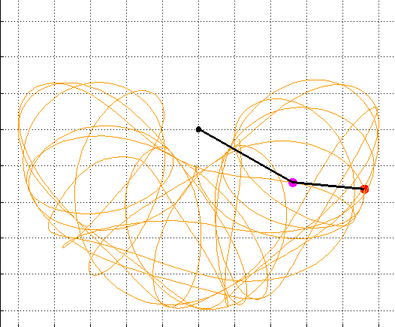
I've always thought that the double-pendulum makes an interesting system to simulate because the problem of doing so sits at the intersection of physics, mathematics, and computer science. The double-pendulum is also an approachable example of a chaotic system, which means it exhibits very complex and interesting behavior. Since I find it so interesting, I'll spend the next few posts writing about the topic. I'll start in this post with a derivation of the equations of motion and a look at the methods used to solve these equations. In the next post we'll actually solve these equations and implement the simulation in a few different programming languages, drawing performance and other comparisons along the way. Post 3 will wrap up this series with a deeper look into the complexities of the system, including an examination of its chaotic properties
Double Pendulum Equations
The equations of the double-pendulum are not for the faint of heart. They actually cannot be solved outright for a closed-form answer, like $(x, y) = f(dx, dy)$. To solve them, numerical methods have to be used. These numerical methods boil down to iterating over very fine time intervals and using simple linear-approximations to solve for small movements in the motion of the both pendulums. You can think of it like trying to draw a curve with a large number of short lines; If you make the lines short enough they appear the same as a true curve from a short distance away. Note that we are not including any resistive forces, whether it be wind resistance or friction in the hinges of the pendulum. One final simplification is that all of the mass of the individual pendulums is contained inside a single point at the end of the rod (every physics lesson needs a cylindrical chicken). In this sense, we are simulating an idealized double-pendulum, the amount of energy it starts with will be the same amount of energy it finishes with and carries throughout the entire simulation. The two pictures below will be used to derive the kinematics and force equations for the double-pendulum.
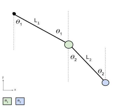
Position Diagram - This diagram is used to derive the kinematics of the system.
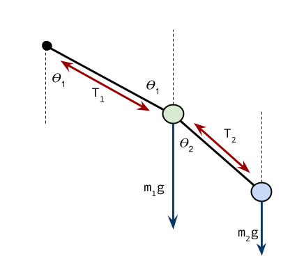
Force-Diagram - This is used to determine the forces on the two masses in terms of gravity and tension in the rods.
Derivation
Big thanks to myphysicslab for their help with the following derivation. To start, let's get the position of both pendulums in terms of the the angles and lengths of the rods (from here on the top pendulum will have subscript 1 and the bottom will have subscript 2). We can then use some calculus to solve for the velocity and acceleration by taking the first and second derivatives of the position equations, making sure to use the chain-rule along the way. I will use the standard 'prime' notation to represent derivatives, as it is slightly more space effecient than the $dx$ notation. Note that the point of all of the following steps is to solve for $\theta_1''$ and $\theta_2''$ in terms of the physical characteristics of the system. In the end, this will allow us to obtain the values for $\theta_1$ and $\theta_2$ over any given time-span from our numerical differential equation solver.
Kinematics Equations
| Trait | x-coordinates | y-coordinates |
|---|---|---|
| Position | $ x_1 = L_1 \sin(\theta_1) $ | $ y_1 = -L_1 \cos(\theta_1) $ |
| $ x_2 = x_1 + L_2 \sin(\theta_2) $ | $ y_2 = y_1 - L_2 \cos(\theta_2) $ | |
| Velocity | $ x_1' = \theta_1' L_1 \cos(\theta_1) $ | $ y_1' = \theta_1' L_1 \sin(\theta_1) $ |
| $ x_2' = x_1' + \theta_2' L_2 \cos(\theta_2) $ | $ y_2' = y_1' - \theta_2' L_2 \sin(\theta_2) $ | |
| Acceleration | $ x_1'' = -L_2\theta_1'^2\sin(\theta_1)+L_2\theta_1''\cos(\theta_1)$ | $ y_1'' = L_2\theta_1'^2\cos(\theta_1)+L_2\theta_1''\sin(\theta_1)$ |
| $ x_2'' = x_1''-L_2\theta_2'^2\sin(\theta_2)+L_2\theta_2''\cos(\theta_2) $ | $ y_2'' =y_1'' + L_2\theta_2'^2\cos(\theta_2)+L_2\theta_2''\sin(\theta_2) $ |
The above equations of kinematics are only about half the battle, we now need to come up with the force equations for the double pendulum. Once we have the force equations, we can balance them with respect to the above equations of kinematics and come out with a form that is suitable for solving numerically.
We'll start with the upper-pendulum, $m_1$. There are 3 forces on this mass, all active in the x-y plane. They consist of the tension from the rod above ($T_1$), the tension from the rod below ($T_2$), and finally the force of gravity ($m_1g$). There are only two forces on the bottom pendulum, and the tension pulling up is just the negative of the tension vector pulling $m_1$ down. Thus the two forces are ($-T_2$) and $m_2g$, the force of gravity. We then have to decompose the forces into their $x$ and $y$ components using trigonometry over the angles $\theta_1$ and $\theta_2$. This leaves us with 4 equations related to the forces of the double pendulum, one in both the $x$ and $y$ directions for both the upper and lower masses. These equations tell us the net force on either object given the individual forces present in the system, and since force is related to acceleration by the famous equation below, we can relate the forces on the objects to our above equations for acceleration. $$ \mathbb{F_{net}} = m\frac{d^2x}{dt^2} $$
Force Equations
| Step # | x-coordinates | y-coordinates |
|---|---|---|
| 1 | $ m_1x_1'' = -T_1 \sin(\theta_1)+T_2 \sin(\theta_2) $ | $ m_1y_1'' = T_1 \cos(\theta_1) - T_2 \cos(\theta_2) - m_1g $ |
| 2 | $ m_2x_2'' = -T_2 \sin(\theta_2) $ | $ m_2y_2'' = T_2 \cos(\theta_2) - m_2g $ |
| 3 | $ T_1 \sin(\theta_1)\cos(\theta_1) = -\cos(\theta_1)(m_1x_1'' + m_2x_2'') $ | $ T_1 \sin(\theta_1)\cos(\theta_1) = \sin(\theta_1)(m_1y_1'' + m_2y_2'' + g(m_1+m_2)) $ |
| 4 | $ T_2 \sin(\theta_2)\cos(\theta_2) = -\cos(\theta_2)(m_2x_2'') $ | $ T_2 \sin(\theta_2)\cos(\theta_2) = \sin(\theta_2)(m_2y_2'' + gm_2) $ |
Steps number 1 and 2 give us $(x_1'',y_1'')$ and $(x_2'',y_2'')$ in terms of the forces of the system. This is not quite what we want, remember we are trying to solve for $\theta_1''$ and $\theta_2''$. To accomplish this we use the kinematics equations derived earlier and some simple algebra. We start by multiplying the $x$ force-equation in step 1 by $\cos(\theta_1)$ and the $x$ force-equation in step 2 by $\cos(\theta_2)$. After that, we strategically combine and rearrange these two to get the x-coordinate equations in steps 3 and 4. Similarly, we multiply the $y$ force-equation in step 1 by $\sin(\theta_1)$ and the $y$ force-equation in step 2 by $\sin(\theta_2)$, then combine and rearrange these two equations to get the y-coordinate equations in steps 3 and 4.
After this, we can set the components in step 3 equal to eachother and same with the components of step 4 to get steps 5 and 6 :
| Step # | Equation |
|---|---|
| 5 | $\sin(\theta_1)(m_1y_1'' + m_2y_2'' + g(m_1+m_2)) = -\cos(\theta_1)(m_1x_1'' + m_2x_2'') $ |
| 6 | $ \sin(\theta_2)(m_2y_2'' + gm_2) = -\cos(\theta_2)(m_2x_2'')$ |
We now have equations relating the trig values of $\theta_1$ and $\theta_2$ to the acceleration components of the upper and lower pendulums. Note also that the kinematics equations tell us how the acceleration, velocity, and position are related to $\theta_1$ and $\theta_2$. Using these facts, we can use a program like Mathematica to solve the equations in steps 5 and 6 for $\theta_1''$ and $\theta_2''$ in terms of the constants of the system and $\theta_1$, $\theta_2$, $\theta_1'$, and $\theta_2'$. Doing just that yields the following two glorious (or hideous, depends on your worldview) equations :
| Step # | Equations |
|---|---|
| 7 | |
8 | $ \theta_2'' = \frac{2\sin(\theta_1-\theta_2)(L_1(m_1+m_2)\theta_1'^2+\cos(\theta_1)g(m_1+m_2) + L_2m_2\theta_2'^2\cos(\theta_1-\theta_2))}{L_2(2m_1+m_2(1-cos(2(\theta_1-\theta_2))))}$ |
There is one final step before we are finished with the derivation. The numerical method we are using to solve these differential equations can only accept first order differential equations (like $x' = f(x)$), so we have to turn this system of 2 second-order equations into a system of 4 first-order equations. We can do this by a simple substitution of variables, letting $\theta_n'$ be $\omega_n$, and thus $\theta_n'' = \omega_n'$ for $n$ in ${[1, 2]}$. This leaves us with the four first-order non-linear differential equations :
| Step # | Final Equations |
|---|---|
| 9 | $\theta_1' = \omega_1$ |
| 10 | $\theta_2' = \omega_2$ |
| 11 | |
12 | $ \omega_2' = \frac{2\sin(\theta_1-\theta_2)(L_1\omega_1^2(m_1+m_2)+\cos(\theta_1)g(m_1+m_2) + L_2m_2\omega_2^2\cos(\theta_1-\theta_2))}{L_2(2m_1+m_2(1-cos(2(\theta_1-\theta_2))))}$ |
The Runge-Kutta Methods
We have now arrived at a point where the equations of motion are suitable for being solved via numerical methods. To accomplish this, we will use a method from the Runge-Kutta family known as RK4 (or The Runge-Kutta Method). This family describes general techniques for approximating the solution to equations of the form : $x' = f(t, x)$. Notice that the rate of change of the state value $(x')$ depends only on the current state and other constants or independent variables (like time or mass). We need equations in this form because they reveal precisely how the system is changing given its current state. This allows us to compute the next state by extrapolating a change in the system over a very small time interval ($h = \delta t$) given only the information that is currently present. We can repeat this process ad infinitum, and as long as our $h$ is small enough, our simulation will remain accurate. Often we need to have more than one equation of the above form to completely describe our system. In this case, we just just treat the components of the above equation as column vectors, resulting in the following equation :
The Runge-Kutta form a family of methods because they assert different but related ways of going about approximating a solution to equations of the above form. The methods in this family of solutions range from relatively-innaccurate but computationally-trivial to very-accurate but slightly more computationally complex. The RK4 is somewhere in the middle, taking a weighted average of the rate of change at 4 different points for each interval to compute the next state. This is shown in the picture below : notice the 4 different tangent lines shown in different colors, which represent the 4 points at which the value of $\textbf{f}(t, \textbf{x})$ is sampled. These slopes are then weighed together, with an emphasis put on the points in the middle, to get a sort of average slope for the interval. If we were working with systems that are more complex than a double-pendulum, a different member from the Runge-Kutta family that takes more samples per interval may be preferable.
RK4 Definition
Let's say we want to compute the values of the state vector $\textbf{x}$ over some period $[t_o, t_f]$ using intervals of time $h$, given that the rate of change ($\textbf{x}'$) is determined by some vector of functions $\textbf{f}(t, \textbf{x})$. We then define the following sequence in which the state during the $n_{+1}$ time interval depends only on the state in the $n_{th}$ interval directly preceding it :
| $\textbf{K}_{1n} = \textbf{f}(t, \textbf{x}_n)$ | $\textbf{K}_{2n} = \textbf{f}(t+\frac{h}{2}, \textbf{x}_n + \frac{h}{2}\textbf{K}_{1n})$ |
| $\textbf{K}_{3n} = \textbf{f}(t+\frac{h}{2}, \textbf{x}_n + \frac{h}{2}\textbf{K}_{2n})$ | $\textbf{K}_{4n} = \textbf{f}(t+h, \textbf{x}_n + h \textbf{K}_{3n})$ |
Given a $\delta t = h$, the state values will correspond to the following times intervals $[t_0, t_0+h, t_0+2h, \ldots, t_f]$. Each state value is computed as the last state value plus some combination of the rates of change that are sampled during the current time interval. This combination is a weighted average of the rate of change at the beginning, middle, and end of the time-span between the $n_{th}$ and the $n-1_{st}$ time intervals. We start by finding the slope at the beginning of the time interval, $\textbf{K}_{1}$. We use this slope value to approximate what the value of $\textbf{x}$ is at $t = t_0+\frac{h}{2}$, labeled $\textbf{K}_2$. We plug these values of $\textbf{x}$ and $t$ into $\textbf{f}$ to get another slope, which is used in the same manner to get $\textbf{K}_3$. The slope value $\textbf{K}_3$ is then used to approximate the value of $\textbf{x}$ at $t = t_0+h = t_1$, giving us $\textbf{K}_4$. These four slope values are weighed together to obtain a sort of average slope for the interval, with an emphasis put on the slope values in the middle ($\textbf{K}_2$ and $\textbf{K}_3$). This average slope is finally used to compute the state at the next time value, $t_1 = t_0 + h$, by taking the last state value plus the average slope multiplied by the time differential. In the picture on the right, notice how we start at the black-dot and end at the pink-dot, slightly off the actual value of $\textbf{x}(t)$.
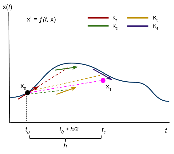
RK4 Approximation - This shows the 4 different places that are used to approximate the change over a short time interval using the RK4 method.
The results we obtain from RK4 are different than if we were able to obtain a closed form solution of $\textbf{x} = [f_1(t), f_2)] $, which would give us the exact state values at any time $t$. To get the state values at a time $t$ using RK4, we have to build up the sequence of states from time $t_0$, with possible innacuracies being introduced during each step. We don't have the luxury of jumping to the exact value of any given state like a closed-form solution would give us. If this all seems a little abstract, we'll make it concrete in the next subsection with a simple example.
Simple Example
Imagine you have a vector of functions $\textbf{f }$ that tells you exactly what the $(dx\text{ , } dy)$ velocity of an object will be at any point in a plane. You also have starting point in the plane $(1, 0)$ for the object :
| step (n) | $ t $ | $\textbf{p}_n$ | $\textbf{K}_{1n}$ | $\textbf{K}_{2n}$ | $\textbf{K}_{3n}$ | $\textbf{K}_{4n}$ | $\textbf{p}_{n+1}$ |
|---|---|---|---|---|---|---|---|
| 1 | 0.0 | (1.0, 0.0) | (2.0, 1.0) | (2.25, 1.15) | (2.283, 1.172) | (2.574, 1.352) | (1.226, 0.116) |
| 2 | 0.1 | (1.226, 0.116) | (2.569, 1.348) | (2.893, 1.551) | (2.936, 1.581) | (3.314, 1.823) | (1.518, 0.273) |
| 3 | 0.2 | (1.518, 0.273) | (3.308, 1.818) | (3.73, 2.091) | (3.785, 2.132) | (4.278, 2.458) | (1.893, 0.484) |
| 4 | 0.3 | (1.893, 0.484) | (4.27, 2.452) | (4.82, 2.82) | (4.893, 2.875) | (5.536, 3.314) | (2.378, 0.769) |
| 5 | 0.4 | (2.378, 0.769) | (5.525, 3.306) | (6.243, 3.802) | (6.34, 3.876) | (7.181, 4.469) | (3.007, 1.153) |
| 6 | 0.5 | (3.007, 1.153) | (7.167, 4.458) | (8.106, 5.127) | (8.234, 5.227) | (9.336, 6.026) | (3.823, 1.671) |
| 7 | 0.6 | (3.823, 1.671) | (9.317, 6.012) | (10.549, 6.913) | (10.718, 7.049) | (12.166, 8.126) | (4.886, 2.369) |
| 8 | 0.7 | (4.886, 2.369) | (12.141, 8.106) | (13.76, 9.322) | (13.983, 9.505) | (15.888, 10.958) | (6.272, 3.31) |
| 9 | 0.8 | (6.272, 3.31) | (15.855, 10.931) | (17.987, 12.57) | (18.282, 12.816) | (20.793, 14.776) | (8.085, 4.58) |
| 10 | 0.9 | (8.085, 4.58) | (20.75, 14.739) | (23.561, 16.95) | (23.953, 17.282) | (27.268, 19.924) | (10.459, 6.292) |
| 11 | 1.0 | (10.459, 6.292) | / | / | / | / | / |
Note that row 11 is mostly empty because the $\textbf{K}$ values for that row would be used to calculate the $x$ value at $t = 1.1s$, we only wanted to go to $t = 1.0s$. If you look down the $\textbf{p}_n$ column, you will see all of the values for our state vector during the $[0,1]s$ time interval.
As this was an approximation, the values in the table are not exactly correct, but they are very close considering how large our $h$ value was. The system of differential equations used in this example is relatively trivial to solve by hand if you've taken a differential equations course (or know how to use Wolfram Alpha), and thus we can compare our approximated answers to the closed-form solution given below :
It's surprising to me that even with such a large $h$ value our approximation stays right on-top of the actual values taken from closed-form solution for the majority of our computation. If our function was much more irregular, then a much smaller $h$ value would have to be used in order to maintain this level of accuracy. The code to generate the points used for the graph above is given below. This is a trivial, non-general implementation in python, in the next post we'll make much more robust implementations.
import math

# this method is our f(x), it returns the slope given the current x,y coordinated
def funt(x, y):
    return (2*x+y, 3*y+1)

# this method returns the closed form solution at time t for comparison
def actual(t):
    x = 0.166666*(3*math.exp(2*t)+2*math.exp(3*t)+1)
    y = 0.3333333*(math.exp(3*t)-1)
    return (x,y)

# performs the next iteration of Runge-Kutta-4
def getNext(x, y, h):
    K1 = funt(x, y)
    x1 = x+K1[0]*h/2
    y1 = y+K1[1]*h/2
    K2 = funt(x1, y1)
    x2 = x+K2[0]*h/2
    y2 = y+K2[1]*h/2
    K3 = funt(x2, y2)
    x3 = x+K3[0]*h
    y3 = y+K3[1]*h
    K4 = funt(x3, y3)

    k = (x+0.166666666*(K1[0]+2*K2[0]+2*K3[0]+K4[0])*h, y+0.166666666*(K1[1]+2*K2[1]+2*K3[1]+K4[1])*h)
    return k

# starting x,y values
p = [(1,0)]
h = 0.1

# end time
end = int(1.1/h)

# runge kutta algorithm
for i in range(0,end):
    p.append(getNext(p[i][0], p[i][1], h))

#print out the computed values
for i in range(0,end):
    t = i*h
    print "[" + str(t) + ", " + str(p[i]) +  "],"

print "\n\n"

# print out the actual values
for i in range(0,end):
    t = i*h
    print "[" + str(t) + ", " + str(actual(t)) +  "],"
This concludes our derivation of the equations of motion of the double-pendulum, as well as our examination of the Runge-Kutta family of methods that will be used to solve them. In the next post, we'll implement RK4 in a few different programming languages and use these implementations to solve this system numerically. Feel free to comment on this post about anything you liked, disliked, or if you you found any errors.
tags : matlab, c++, math, physics, double-pendulum, chaos