Simulating a Double Pendulum - Part 2
2015-03-25
Taking a small break from writing this post to work on the infrastructure for this website. It will be continued soon.
In this post, we build off the theory developed in Part 1 and actually implement a double-pendulum simulator in a few different programming languages. We'll start by writing our own Runge-Kutta solvers which will give us the position, velocity, and acceleration data that is needed to completely describe the trajectory of a double pendulum system given an arbitrary set of initial conditions. Once we have this data, we can move onto plotting it using a few different plotting libraries. The languages I'll be going over are Matlab, C++, and Python. I chose these languages because they are all quite popular and any given programmer is likely to understand at least one of them.
Getting the Code
All of the code is hosted here on Github, and more details can be found at the Double-Pendulum-Simulation project page on my website. The entire project is available for download via either of these two links : .Tar , .Zip. You can also clone it straight from the command line :
git clone https://github.com/jhallard/Double-Pendulum-Simulation.git
cd Double-Pendulum-Simulation
Quick Review
Below is a quick summary of the last post, for more information, read Part 1.
- Expand Section
Below are the 4 differential-equations describing the motion of the masses on ends of the upper and lower pendulums.
1 $\theta_1' = \omega_1$ 2 $\theta_2' = \omega_2$ 3 $\omega_1' = \frac{-g(2m_1 + m_2)\sin(\theta_1) - m_2g\sin(\theta_1 - 2\theta_2) - 2\sin(\theta_1 - \theta_2)m_2(L_2\omega_2^2+L_1\omega_1^2\cos(\theta_1 - \theta_2))}{L_1(2m_1+ m_2(1 - \cos(2(\theta_1-\theta_2))))} $ 4 $ \omega_2' = \frac{2\sin(\theta_1-\theta_2)(L_1\omega_1^2(m_1+m_2)+\cos(\theta_1)g(m_1+m_2) + L_2m_2\omega_2^2\cos(\theta_1-\theta_2))}{L_2(2m_1+m_2(1-cos(2(\theta_1-\theta_2))))}$ Here is the definiton of the Runge-Kuta-4 method.
$$ \textbf{x}_{n+1} = \textbf{x}_n + \frac{h}{6}(\textbf{K}_{1n} + 2\textbf{K}_{2n} + 2\textbf{K}_{3n} + \textbf{K}_{4n})$$ $$ t_{n+1} = t_n + h $$The 4 values $\textbf{K}_{1n}, \textbf{K}_{2n}, \textbf{K}_{3n}, \textbf{K}_{4n}$ are defined as follows :$\textbf{K}_{1n} = \textbf{f}(t, \textbf{x}_n)$ $\textbf{K}_{2n} = \textbf{f}(t+\frac{h}{2}, \textbf{x}_n + \frac{h}{2}\textbf{K}_{1n})$ $\textbf{K}_{3n} = \textbf{f}(t+\frac{h}{2}, \textbf{x}_n + \frac{h}{2}\textbf{K}_{2n})$ $\textbf{K}_{4n} = \textbf{f}(t+h, \textbf{x}_n + h \textbf{K}_{3n})$ Matlab
Matlab is a proprietary language, which means you'll have to buy the software to be able to use this implementation. What we get in exchange for this purchase is a very complex and thorough library of built-in functions, including some wonderful implementations of the Runge-Kutta algorithms. This makes our job extremely simple, all we need to do is define the system of equations and pass them to a library function called
ode45, which will return a series of parallel arrays containing all of the data needed for the plots. I'll start by going over how to define the equations of motion that need to be solved, then move onto making the simulation code, and finish by showing the results of our program.Equations
The first file I made is
DoublePendEquations.m. The purpose of this file is to hold a single function that returns a vector of equations, the differential equations defined in the table above.DoublePendEquations.mfunction xdot = DoublePendEquations(t, ic) %extract the initial conditions from the ic vector theta1 = ic(1); dtheta1 = ic(2); theta2 = ic(3); dtheta2 = ic(4); grav=ic(5); m1=ic(6); m2=ic(7); len1=ic(8); len2=ic(9); xdot=zeros(9,1); %theta1 prime = angular velocity1 xdot(1)=dtheta1; % angularvelocity1 prime = this equation xdot(2)= -(grav.*(2*m1+m2)*sin(theta1) + m2*grav*sin(theta1-2*theta2)... + 2*sin(theta1-theta2)*m2*((dtheta2.^2)*len2 + (dtheta1.^2).*len1*cos(theta1-theta2))) / (len1*(2*m1+m2-m2*cos(2*theta1-2*theta2))); %theta2 prime = angular velocity2 xdot(3)=dtheta2; %angularvelocity2 prime = this equation xdot(4)= (2*sin(theta1-theta2)*((dtheta1.^2)*len1*(m1+m2)+grav*(m1+m2)*cos(theta1)... +(dtheta2.^2)*len2*m2*cos(theta1-theta2)))/... (len2*(2*m1+m2-m2*cos(2*theta1-2*theta2))); endThis function (
DoublePendEquations) takes in two arguments, the first being a value for the time, labeledt. The next is a vector of initial conditions, appropriately labeledic. This vector contains values for all of the constants of the system (like the masses, lengths, etc) as well as the initial starting positions and initial velocities for the pendulums. These values entirely describe the starting state for our system, which in-turn can be used to calculate exactly how the system will evolve as time goes forward. Matlab is nice in that it is very high level, and thus we can simply assign each of the 4 equations to their own variables in a symbolic fashion. This allows us to keep the programming very close to the theory that was derived; notice that we have a literal vector of symbolic equations, which is exactly what the theory behind the Runge-Kutta-4 algorithm requires. In lower-level languages like C++, the code won't as closely resemble the theory, and we'll have to perform some slight tricks to get everything working.Solving with
ode45.Since we're using Matlab it wouldn't be worth our time to implement our own Runge-Kutta algorithm, there are many built into the software that are much more robust than anything we could write. As the Runge-Kutta methods are a family of methods with different accuracies and computational complexities, Matlab provides a few different versions for our use. The most popular is
With the function defined in file above, we can now solve the system of equations in just a few calls to library-functions. In the code defined in this project, there are 4 different simulation functions,ode45, which is the one we will be using. This algorithm is the most widely-used and considered the most accurate RK method to use, but it only applies to 'non-stiff' differential equations. Stiff equations are exactly those which fail to be accurately solvable using traditional numerical methods, and they are equations describing the most sensitive of systems, much more sensitive than our already hyper-sensitive double-pendulum (sensitivity to initial conditions will be discussed in part 3).DoublePendSimulationXfor X as nil and 1-3. Each one takes the same arguments but displays different graphs, more on that in a later section. The code to useode45is given below.DoublePendSimulation3.mfunction DoublePendSimulation3(ic, time) %define the normal frames per second of the animation and the adjusted fpsnormal = 30; fps = fpsnormal*1.0; numframes=time*fps; %define the tolerances for the ode45 method options = odeset('Refine',6,'RelTol',1e-5,'AbsTol',1e-7); %solve the differential equations defined in the function @DoublePendEquations, %over the interval t = 0 to t = time, with the initial conditions specified %in the vector ic, according to the options defined directly above. solutionsstruct=ode45(@DoublePendEquations,[0 time], ic, options); %define a discrete vector of points that we want to obtain the solutions on t = linspace(0,time,numframes); %extract the system-state values defined on the linespace above solutionsvector=deval(solutionsstruct,t); % get the individual components of the solution vector theta1=solutionsvector(1,:)'; angvel1=solutionsvector(2,:)'; theta2=solutionsvector(3,:)'; angvel2=solutionsvector(4,:)'; %get the individual initial conditions and constants passed in by the user len1=ic(8); len2=ic(9); m1 = ic(6); m2 = ic(7); moment1 = 0.5.*m1.*len1.^2; moment2 = 0.5*m2.*len2.^2; grav = ic(5); % ... continued below ...The
DoublePendSimulation3function is the one called by the user to actually solve a double-pendulum system given a set of initial conditions. It takes in our vector of initial conditions (defined by an input-vector that the user submits when they call the function) and an ending time for the simulation, which always start att=0seconds. We start by defining some error tolerances for theode45function, which boil down to telling it how small to make the $\delta t = h$ time interval that we approximate over. Next is our actual call toode45. The first argument is a reference to our function that defines the differential equations,DoublePendEquations. The@symbol in Matlab is used to reference functions, like a function-pointer in the C languages. We then pass in a vector containing the start and end time of the simulation, along with the vector of intial conditions passed-in by the user and finally the options that were defined above.Our call to ode45 can return various types of values depending on the structure of the variable we assign the return value to (described in detail here). In this case, we are returned a structure from which state-values can be extracted. To do this extraction, we use the
devalfunction over a discrete number oftvalues, which are generated with thelinspacefunction. This allows us to extract only the state-values at intervals equal to our frame-rate, instead of getting values every $10^{-6}$ seconds (which is the discretization of our solution). The next 8 lines of code extract the individual components of the macro-state into appropriately-named variables, which will make the rest of our code more clean and explicit. Notice that thetheta1variable is the first row of solutions returned, which corresponds to $\theta_1'$ being the first element in the vector of equations we defined in@DoublePendEquations. The same applies to the variablestheta2, angvel1, angvel2, all of the first-order differential equations have now turned into vectors of values giving the trajectory of the system.Creating the Simulation
Matlab's built-in libraries will once again be very useful here, as making a simulation is sometimes as easy as a single function call placed inside of a for-loop. Ours will be a bit more complicated, most of the overhead being cosmetic-related code. Since we have all of this data, we are able to do a bit more than just show the positions of the pendulums through time, we can also show graphs of the angles, perform an energy analysis, and graph many other metrics. I'll start below by giving the code just to simulate the actual motion of the double-pendulum.
We start by defining a figure and a subplot inside of that figure. We then define a few different types of plots that are going to go inside this subplot bounding-box. These consist of a line plot for the pendulum rods, a scatter-plot to make the two objects at the end of the rods, and finally another line plot to show the $(x,y)$ coordinates of the bottom mass over time. All of the vectors we are using to hold the plotting data are initialized so they don't have to be resized during each iteration of the loop. We then turn the theta values into $(x,y)$ coordinates by using some trigonometry, which puts all of our data in a form ideal for the simulation loop. The main for-loop is relatively simple, we just set the $x$ and $y$ data for each plot to the appropriate coordinate values that we previously calculated, draw the frame, and watch the simulation unfold.
DoublePendSimulation3.m(continued)% Continuing from the last section of code, above... % %initialize vectors to hold the x and y coordinated of the lines we are %going to be plotting linex1 = zeros(0, numframes-1); linex2 = zeros(0,numframes-1); liney2 = zeros(0,numframes-1); liney1 = zeros(0, numframes-1); timearr = zeros(0,numframes-1); %create the figure window, set it to outer edges of screen figure('units','normalized','outerposition',[0 0 1 1]); % this subplot defnes the coordinates and size of the pendulum pos. plot subplot('Position',[.1 .1 .8 .8]);hold on; % this plots the line that shows where the bottom pendulum has been pendline = plot([0 0], [0 0], 'Color', [1 153/255 0]); %h is the handle to the actual plot of the 2 pendulums x and y coordinates rods = plot(0,0,'k', 'LineWidth',2); ColorSet = [0 0 0; 1 0 1; 1 0 0]; %this plot places the objects on the ends up the pendulums pendobjects = scatter([0 0 0], [0 0 0], [50, 100, 100], ColorSet, 'filled'); axis equal;grid on; title('Double Pendulum Motion', 'fontweight', 'bold', 'fontsize',10); hold off; %set axis limits to just outside of the double-pends reach range=1.1*(len1+len2); axis([-range range -range range]); %turn the theta values into x/y valuyes for both pendulums linex1 = len1*sin(theta1); liney1 = -len1*cos(theta1); linex2 = linex1+len2*sin(theta2); liney2 = liney1-len2*cos(theta2); %simulation loop for i=1:numframes timearr(i) = i/fps; Xcoord=[0,linex1(i),linex2(i)]; Ycoord=[0,liney1(i),liney2(i)]; %pendulum position simulation set(pendline,'XData',linex2(1:i),'YData',liney2(1:i)); set(rods,'XData',Xcoord,'YData',Ycoord); set(pendobjects,'Xdata', Xcoord, 'YData', Ycoord); drawnow; end endSimulation Results
The code includes 4 different simulations/combinations of simulations, and is run from the matlab command line as described below. I am able to get 30+ FPS running 32bit Matlab 2012a Student on Ubuntu 14.04 64bit, so I suspect it would run faster on a more appropriate set-up. Matlab's dynamic typing, rich libraries, and symbolic-math support made this the easiest program to write and write-about. It would have been interesting to implement our own RK4 instead of using
ode45, but the robustness and simplicity of the built-in function made the thought of implementing my own too boring to spend my time on.Getting it Running
Follow these instructions to use the simulator on your computer.
Clone the file from Github if you haven't already.
  git clone https://github.com/jhallard/Double-Pend-Simulation.git
  cd Double-Pend-Simulation
Open up Matlab, I was using version 2012A Student, but any newer version should also work just fine. Navigate to
Double-Pendulum-Simulation/matlab/as your working directory. You will be calling one of theDoublePendSimulationX()functions, and passing in 3 arguments, one of them being a vector of arugments itself. The 3 arguments are :- IC - Initial conditions vector.
ic = [theta1;angvel1;theta2;angvel2;grav;mass1;mass2;len1;len2;] - time - The ending time of the simulation.
- simspeed - A factor by which to slow-down the simulation, i.e. 2.0 means twice as slow.
Try one of the following function calls :
  DoublePendSimulation3([.849;-.2;-1.35;0.0;9.81;0.9;.7;.6;.4],55,1.0, 2);
  DoublePendSimulation4([.75;-.2;-.1.15;0.0;9.81;0.9;.7;.6;.4],35,1.0, 2);
Examples
Below are two screen-shots from this simulation, I'm in the process of making GIFs but Matlab isn't being very compliant on Linux right now.
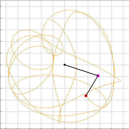
Matlab Simulation - Run #1, a large amount of initial energy.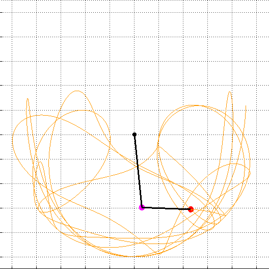
Matlab Simulation - Run #2, less initial energy put into the system.C++
The C++ implementation was the most time-consuming of the three to make, but it was also my favorite. I chose to start by creating a simple class-hierarchy that serves as a wrapper around a given set of equations. This wrapper provides a well-defined interface that our Runge-Kutta implementation will be programmed to work with. The user can simply derive and override this equation-wrapper class as many times as they please, and as long as they return the values via the defined interface everything will work. This hierarchy will have
FunctionWrapperRK4as its base class, and I will also define a child classDoublePendEquationsthat will be specific to our double pendulum simulation. Once those classes are defined, the general RK4 class can be implemented without too much effort. This RK4 class will be able to accept any class in thisFunctionWrapperRK4hierarchy and solve the equations using the Runge-Kutta-4 algorithm. After the code to solve the system in finished, I go over making the simulation with the matplot++.Equations
To define the classes I decided on building a base class which can wrap around a given set of equations. The RK4 class that will be examined in the next section can then access all sets of user-defined functions through the interface defined by the wrapper-class. These classes represent vectors of functions, a loose mathematical concept that makes plenty of sense while programming. The number of functions that the class wraps around is decided by the user and not bounded by the class itself.
FunctionWrapperRK4
The FunctionWrapperRK4 serves as a simple base class. It only holds the number of equations needed to describe the system and provides the
getValuesfunction as a template that must be overwritten by child classes. This is done by making it bothvirtual, which allows it to be overwritten, and= 0, which explicitely states it has no definition, so a child won't compile without overwritting it.FunctionWrapperRK4.h#ifndef FUNC_WRAP_RK4 #define FUNC_WRAP_RK4 #include <vector> #include <cmath> // @class - FunctionWrapperRK4 // @info - This is to serve as the base class for this hierarchy. All of these classes are meant to be // wrappers around sets of equations that are passed into the RK4 class to be solved. class FunctionWrapperRK4 { private: // number of equations to wrap with this object int _num_equations; public: // @func - Constructor // @args - #1 number of equations to be wrapped FunctionWrapperRK4(int); // @func - getValues // @args - #1 current time value to be used #2 current state values to be used // @info - Overwritte this with child classes to return the true function values. virtual std::vector<double> getValues(double, const std::vector<double> &) = 0; // @self-documenting int getNumEquations() const; }; #endifThe definition for the constructor, the
getValuesfunction, and an access function for the number of equations are included in their own fileFunctionWrapperRK4.cpp. This class is made very simple on-purpose, to minimizes any un-necessary restrictions put on the classes that will dervive from this one.FunctionWrapperRK4.cpp#include "FunctionWrapperRK4.h" FunctionWrapperRK4::FunctionWrapperRK4(int num_equations) { if(num_equations >= 1) _num_equations = num_equations; } int FunctionWrapperRK4::getNumEquations() const { return _num_equations; }DoublePendEquations
Now that a proper base-class is defined, the next step is to define a child class that is specific to our double-pendulum system. This class is called
DoublePendEquations, it contains any and all data/functions that we think are necessary to compute the values described by the equations of motion. I start by adding private member variables to represent the constants of the system : gravity, the two masses, and the two lengths. These values will be set by the user when the constructor is called and can't be changed after this. Then I added variables to hold the current state-values, which are the two angles and two angular velocities (upper and lower for each). Along with a passed-in time value, this is enough data to determine what the values of our four differential-equations are over any combination of valid input. For thegetValuesfunction, instead of defining the four equations in-line, I broke it up into 4 seperate member-functions. These 4 functions (upperThetaPrime,lowerThetaPrime,upperOmegaPrime,lowerOmegaPrime) take the current time and return the value for that specific differential equation. The values from these 4 functions are aggregated, placed into a vector by thegetValuesfunction, and returned as was specified via theFunctionWrapperRK4interface.All of the constants for our double-pendulum system have to be positive (gravity, length, and mass all are positive), so any negative values passed into a constructor will cause an exception to be thrown. Our class is assuming SI units (meters) and that we are working in radians instead of degrees. The
getValuesfunction takes in the current state-values and assigns them to the appropriate member variables before calling the 4 differential-equations and putting the values in a vector in the same order that the state-values arrive.DoublePendEquations.h#ifndef DOUBLE_PEND_EQUATIONS_JHA #define DOUBLE_PEND_EQUATIONS_JHA #include "FunctionWrapperRK4.h" #include <stdexcept> // @class - DoublePendEquations // @info - This class is a child class of the FunctionWrapperRK4 base class, and is used to represent the differential-equations of // motions for a double-pendulum in a manner that allows them to be solved by our implementation of the Runge-Kutta-4 // method (@file RK4.h). class DoublePendEquations : public FunctionWrapperRK4 { private: // system constants (u-prefix is upper l-prefix is lower) double _gravity, _length1, _mass1, _length2, _mass2; // specific state values that are extracted from the given state vector double _theta1, _theta2, _omega1, _omega2; // @func - upperThetaPrime // @info - This is the differential equation for the upper theta variable : theta1' = omega1 double upperThetaPrime(double time); // @func - upperThetaPrime // @info - This is the differential equation for the lower theta variable : theta2' = omega2 double lowerThetaPrime(double time); // @func - upperThetaPrime // @info - This is the differential equation for the upper omega (angular velocity) variable : omega1' = 2sin(theta_1-theta_2)... double upperOmegaPrime(double time); // @func - upperThetaPrime // @info - This is the differential equation for the upper omega (angular velocity) variable : omega2' = L1cos(theta_1-theta_2)... double lowerOmegaPrime(double time); public: // @func - Constructor // @args - #1 vector of values for the constants above DoublePendEquations(std::vector<double>); // @func - Constructor #2 // @args - explicit values for constants above DoublePendEquations(double gravity, double length1, double mass1, double length2, double mass2); // @func - getValues // @args - #1 current time value to be used in the calculations, #2 vector of values for the 4 changing state variables (uangle, // uangvel, langle, langvel) // #info - This function is simply going to call the 4 private utility functions to get the values, it exists to fufill the interface defined // by the base class in the hierarchy. virtual std::vector<double> getValues(double, const std::vector<double> &); }; #endifBelow is the definition of the
DoublePendEquationsclass. There isn't too much going on here, just a decent amount of input-validation to ensure that the system makes physical sense and that the incoming state-values are in the correct form. I use the standard underscore-prefix for member variables, and mixed-case for class names.DoublePendEquations.cpp#include "DoublePendEquations.h" // @func - Constructor // @args - #1 vector of values for the constants above DoublePendEquations::DoublePendEquations(std::vector<double> constants) : FunctionWrapperRK4(4), _theta1(0), _theta2(0), _omega1(0), _omega2(0) { if(constants.size() != 5) { throw std::logic_error( "Error : Initial condition vector needs 5 double values (grav, ulen, umass, llen, lmass)."); } for(auto x : constants) { if(x <= 0) { throw std::logic_error("Error : All system-constant values must be positive."); } } _gravity = constants[0]; _length1 = constants[1]; _mass1 = constants[2]; _length2 = constants[3]; _mass2 = constants[4]; } // @func - Constructor #2 // @args - explicit values for constants above DoublePendEquations::DoublePendEquations(double gravity, double ulength, double umass, double llength, double lmass) : FunctionWrapperRK4(4) , _theta1(0), _theta2(0), _omega1(0), _omega2(0) { std::vector<double> constants = {gravity, ulength, umass, llength, lmass}; if(constants.size() != 5) { throw std::logic_error( "Error : Initial condition vector needs 5 double values (grav, ulen, umass, llen, lmass)."); } for(auto x : constants) { if(x <= 0) { throw std::logic_error("Error : All system-constant values must be positive."); } } _gravity = constants[0]; _length1 = constants[1]; _mass1 = constants[2]; _length2 = constants[3]; _mass2 = constants[4]; } // @func - upperThetaPrime // @info - This is the differential equation for the upper theta variable : theta1' = omega1 double DoublePendEquations::upperThetaPrime(double time) { return _omega1; } // @func - upperThetaPrime // @info - This is the differential equation for the lower theta variable : theta2' = omega2 double DoublePendEquations::lowerThetaPrime(double time) { return _omega2; } // @func - upperThetaPrime // @info - This is the differential equation for the upper omega (angular velocity) variable : omega1' = 2sin(theta_1-theta_2)... double DoublePendEquations::upperOmegaPrime(double time) { double numerator = -1.0*_gravity*(2*_mass1+_mass2)*sin(_theta1) - _gravity*_mass2*sin(_theta1-2*_theta2); numerator = numerator - 2*_mass2*sin(_theta1-_theta2)*(_length2*pow(_omega2, 2)+_length1*pow(_omega1, 2)*cos(_theta1-_theta2)); double denominator =_length1*(2*_mass1+_mass2*(1-cos(2*(_theta1-_theta2)))); if(denominator == 0) throw std::logic_error("Error : Denominator 0 in upperOmegaPrime"); return (double) numerator/denominator; } // @func - upperThetaPrime // @info - This is the differential equation for the upper omega (angular velocity) variable : omega2' = L1cos(theta_1-theta_2)... double DoublePendEquations::lowerOmegaPrime(double time) { double numerator = 2*sin(_theta1-_theta2); numerator *= (_length1*pow(_omega1,2)*(_mass1+_mass2)*_gravity*cos(_theta1)*(_mass1+_mass2)+_length2*_mass2*pow(_omega2,2)*cos(_theta1-_theta2)); double denominator = _length2*(2*_mass1+_mass2*(1-cos(2*(_theta1-_theta2)))); if(denominator == 0) throw std::logic_error("Error : Denominator 0 in lowerOmegaPrime"); return (double)numerator/(double)denominator; } // @func - getValues // @args - #1 current time value to be used in the calculations, #2 vector of values for the 4 changing state variables (uangle, // uangvel, langle, langvel) // #info - This function is simply going to call the 4 private utility functions to get the values, it exists to fufill the interface defined // by the base class in the hierarchy. std::vector<double> DoublePendEquations::getValues(double curr_time, const std::vector<double> & state) { if(state.size() != 4) { throw std::logic_error("Error : state-vector must contain 4 double values (theta1, theta2, omega1, omega2."); } _theta1 = state[0]; _theta2 = state[1]; _omega1 = state[2]; _omega2 = state[3]; std::vector<double> diffeq_values; diffeq_values.push_back(upperThetaPrime(curr_time)); diffeq_values.push_back(lowerThetaPrime(curr_time)); diffeq_values.push_back(upperOmegaPrime(curr_time)); diffeq_values.push_back(lowerOmegaPrime(curr_time)); return diffeq_values; }It's important to note that an order to the equations must be chosen, as this is the same order that the solved state-values will be passed into the function. In our case, the ordering is $\theta_1', \theta_2', \omega_1', \omega_2'$ as the 1st-4th differential equations, thus the solved state-vectors will have the ordering
_theta1,_theta2,_omega1,_omega2. One other thing I would like to point out is we could have defined as many equations as we wanted using any arbitrary data-types as members of our class, all we would have to do is round up the values from our various functions and place them into a vector to be returned via thegetValuesvirtual function. The RK4 class needs to know nothing the equations it is solving in particular, just how many of them their are and that the values will be returned in order from the when the virtual function is called.Runge-Kutta Solver
Now that we have properly defined an interface through which one can access arbitrary equation values (
FunctionWrapperRK4) and implemented a specific instance of that interface (DoublePendEquations), we can move onto building a class to solve a set of equations using the RK4 algorithm. If you aren't familiar with the Runge-Kutta-4 method, see the last post, where I went over it in detail including a simple example.RK4 Class Overview
The entire RK4 implementation is inside of a single class with a simple interface. In order to solve and retrieve the state-values for a given system of differential equations, the following steps are required.
- Wrap the system of equations in a custom class that is derived from the
FunctionWrapperRK4class. Create an instance of the RK4 class, and upon construction pass in the address of an object of your custom equation-wrapper class. - Call the
RK4::solvefunction. This function takes in 3 argument; The discretization for the simulation, the ending time of the simulation (always starts at $t_0=0$), and finally a vector of initial conditions. The vector of initial conditions must be the same size as the number of equations you are solving, and the ordering should correspond the differential equation ordering. This function will solve the system from $t = 0$ to $t = t_f$ with a time-step equal to the disc. passed in. - Query the state-value solutions over specific time intervals. I chose seperate the solving from the data-retrieval because often we need to calculate a much denser sequence of state-values then are needed to make a simulation.For example, we could use a spacing of $0.00001$ seconds to solve the system but we only needs a spacing of $0.01677$ to get 60 frames per second. Simply returning all of the state-values would introduce an unnecessary time-overhead for our simulation
This RK4 class has a pointer to base-class (
FunctionWrapperRK4 *) as a private member. This member will be assigned to point to any child class in the hierarchy upon construction. We use a pointer to base-class because this allows us to use polymorphism, which in short means that our program can determine which virtual function in a hierarchy to call at run-time. Since we want to work with an arbitrary number of equations, we usestd::vectorsas our $\textbf{K}$ values (_k1-_k4). These four vectors are filled for each step of the simulation, and are combined together with the current state-values to get the next set of state-values. During the main RK4 loop in thesolvefunction, every set of state-values is saved into a set of parallel vectors, named_solution. These are the values that are sorted by thequeryfunction to return only the data that the user requires. The declaration of theRK4class is given below.RK4.hclass RK4 { private: int _num_equations; // number of equations to be solved simultaneously double _disc; // discretization step std::vector<double> _k1, _k2, _k3, _k4; // 4 K vectors double _tf; // pointer to base object that serves as our interface to the diff. equations defined by the user FunctionWrapperRK4 * _equations; // vector of vectors, this holds an array of state-values for each of the variables that need to be solved. std::vector<std::vector<double> > _solutions; // @func - stateAdjust // @args - #1 vector to be adjusted, #2 vector to add to the first, #3 constant factor to adjust 2nd vector by std::vector<double> stateAdjust(const std::vector<double> &, const std::vector<double> &, double); // @func - vectorAdd // @info - takes a vector of vectors of the same length and adds all the components together std::vector<double> vectorAdd(std::vector<std::vector<double> > vecs); public: // @func - Constructor // @args - #1 ptr to base class, should hold your derived class that contains the // equations of motion to be solved. RK4(FunctionWrapperRK4 * fn); // @func - solve // @args - #1 discretization, #2 final time for simulation (from 0s), #3 vector of initial condition values bool solve(double disc, double tf, std::vector<double> ic); // @func - query // @args - #1 the starting time for the query, #2 the end time for the query, #3 the time step you wish to jump between those points std::vector<std::vector<double> > query(double t0, double tf, double step); // @func - setEquations // @info - enter a new set of equations to be solved bool setEquations(FunctionWrapperRK4 * fn); // @func - getEquations // @info - get the equations object being used currently. FunctionWrapperRK4 * getEquations(); };Besides the items listed above, we also include a few private functions that let us perform manipulation of arbitrary-sized vectors. We also provide get and set functions for the system of equations being solved, which allows one RK4 class to work with different systems over its life-time. The definition of the class is given below.
RK4.cpp#include "RK4.h" // @func - Constructor // @args - #1 ptr to base class, should hold your derived class that contains the // equations of motion to be solved. RK4::RK4(FunctionWrapperRK4 * fn) { if(fn == nullptr) { throw std::logic_error("Error : FunctionWrapper object must not be null."); } _equations = fn; if(_equations->getNumEquations() <= 0) { throw std::logic_error("Error : Cannot solve system of <1 equations."); } _num_equations = _equations->getNumEquations(); _solutions.resize(_num_equations); } void printKValues(std::vector<std::vector<double> > vals) { int it = 1; for(auto x : vals) { printf("%d : ", it++); for(auto y : x) { printf("%f ", y); } printf("\n"); } } // @func - solve // @args - #1 discretization, #2 final time for simulation (from 0s), #3 vector of initial condition values bool RK4::solve(double disc, double tf, std::vector<double> ic) { if(disc <= 0) { throw std::logic_error("Error : Time step must be > 0."); } _disc = disc; if(tf <= 0) { throw std::logic_error("Error : Ending time must be > 0"); } _tf = tf; if(ic.size() != _num_equations) { throw std::logic_error("Error : Not enough initial conditions Submitted"); } _solutions.clear(); _solutions.resize(_num_equations); std::vector<double> states = ic; int num_steps = (int)tf/disc; // main RK4 loop for(int i = 0; i <num_steps; i++) { double t = i*_disc; for(int i = 0; i <states.size(); i++) { _solutions[i].push_back(states[i]); } _k1 = _equations->getValues(t, states); _k2 = _equations->getValues(t+0.5*disc, stateAdjust(states, _k1, 0.5)); _k3 = _equations->getValues(t+0.5*disc, stateAdjust(states, _k2, 0.5)); _k4 = _equations->getValues(t+disc, stateAdjust(states, _k2, 1.0)); std::vector<std::vector<double> > vals = {_k1, _k2, _k2, _k3, _k3, _k4}; // printKValues(vals); std::vector<double> sum = vectorAdd(vals); states = stateAdjust(states, sum, 0.16666); } return true; } // @func - query // @args - #1 the starting time for the query, #2 the end time for the query, #3 the time step you wish to jump between those points std::vector<std::vector<double> > RK4::query(double t0, double tf, double step) { if(t0 <0 || tf > _tf || step > tf-t0) { throw std::logic_error("Error : Invalid bounds in query"); } int start_index = t0/_disc; if(start_index <0) { start_index = 0; } int end_index = tf/_disc; int jump = step/_disc; std::vector<std::vector<double> > ret(_num_equations); for(int i = start_index; i <end_index && i <_solutions[0].size(); i += jump) { for(int j = 0; j <_num_equations; j++) { ret[j].push_back(_solutions[j][i]); } } return ret; } // @func - setEquations // @info - enter a new set of equations to be solved bool RK4::setEquations(FunctionWrapperRK4 * fn) { if(fn == nullptr) { throw std::logic_error("Error : FunctionWrapper object must not be null."); } _equations = fn; if(_equations->getNumEquations() <= 0) { throw std::logic_error("Error : Cannot solve system of <1 equations."); } _num_equations = _equations->getNumEquations(); _solutions.clear(); _solutions.resize(_num_equations); } // @func - getEquations // @info - get the equations object being used currently. FunctionWrapperRK4 * RK4::getEquations() { return _equations; } // @func - stateAdjust // @args - #1 vector to be adjusted, #2 vector to add to the first, #3 constant factor to adjust 2nd vector by std::vector<double> RK4::stateAdjust(const std::vector<double> & base, const std::vector<double> & adj, double factor) { if(base.size() != adj.size()) { throw std::logic_error("Error : Vector addition requires same size vectors"); } std::vector<double> ret; for(int i = 0; i <base.size(); i++) { ret.push_back(base[i]+adj[i]*factor*_disc); } return ret; } // @func - vectorAdd // @info - takes a vector of vectors of the same length and adds all the components together std::vector<double> RK4::vectorAdd(std::vector<std::vector<double> > vecs) { if(vecs.size() <= 0) { return std::vector<double>(); } int size = vecs[0].size(); std::vector<double> ret; for(auto vec : vecs) { if(vec.size() != size) { throw std::logic_error("Error : Vector addition requires same size vectors"); } } for(int i = 0; i <size; i++) { ret.push_back(0.0); } for(int i = 0; i <vecs.size(); i++) { for(int j = 0; j <vecs[i].size(); j++) { ret[j] += vecs[i][j]; } } return ret; }Solving and Simulating the System
All of the infrastructure needed to solve the equations of motion has now been built, so we can move onto designing the program to actually solve and simulate the double-pendulum system. This will consist of a single program, DoublePendSimulator, that is launched via the command line with a file-name containing simulation options as an argument. The program parses this file of arguments and launches a window to display the simulations. Code-wise, the program is broken up into 2 main parts: mathematics and graphics.
Data Processing
It was now time to combine our
RK4class along with ourDoublePendEquationsclass to give us the state-values of the double-pendulum system over any set of initial conditions. Now that we created a means of getting the data-points for any double-pendulum system we wish, we can move onto plotting this data.Simulation Results
Python
Coming Soon!
Here's some place-holder code from the last blog-post, it performs a comparison between a simple RK4 implementation and the closed-form solutions to a simple system of differential equations.
import math # this method is our f(x), it returns the slope given the current x,y coordinated def funt(x, y): return (2*x+y, 3*y+1) # this method returns the closed form solution at time t for comparison def actual(t): x = 0.166666*(3*math.exp(2*t)+2*math.exp(3*t)+1) y = 0.3333333*(math.exp(3*t)-1) return (x,y) # performs the next iteration of Runge-Kutta-4 def getNext(x, y, h): K1 = funt(x, y) x1 = x+K1[0]*h/2 y1 = y+K1[1]*h/2 K2 = funt(x1, y1) x2 = x+K2[0]*h/2 y2 = y+K2[1]*h/2 K3 = funt(x2, y2) x3 = x+K3[0]*h y3 = y+K3[1]*h K4 = funt(x3, y3) k = (x+0.166666666*(K1[0]+2*K2[0]+2*K3[0]+K4[0])*h, y+0.166666666*(K1[1]+2*K2[1]+2*K3[1]+K4[1])*h) return k # starting x,y values p = [(1,0)] h = 0.1 # end time end = int(1.1/h) # runge kutta algorithm for i in range(0,end): p.append(getNext(p[i][0], p[i][1], h)) #print out the computed values for i in range(0,end): t = i*h print "[" + str(t) + ", " + str(p[i]) + "]," print "\n\n" # print out the actual values for i in range(0,end): t = i*h print "[" + str(t) + ", " + str(actual(t)) + "]," - IC - Initial conditions vector.
tags : matlab, c++, math, physics, double-pendulum, chaos, python